Example Netlists
Here are some example circuits, with the input and output from LTspice. They aren't necessarily realistic electronic circuits but more of a journal of tests performed while the code was developed.
| Netfile | Schematic | LTspice Output | Notes |
|---|---|---|---|
|
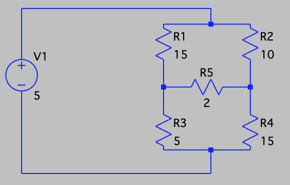
V1 N001 0 5
R1 N001 N002 15 R2 N001 N003 10 R3 N002 0 5 R4 N003 0 15 R5 N002 N003 2 .op .backanno .end |
Wheatstone
|
V(N001) 5.0
V(0) 0 V(N002) 1.81 V(N003) 2.11 I(V1) -0.5 I(R1) 0.21 I(R2) 0.29 I(R3) 0.36 I(R4) 0.14 I(R5) -0.15 |
A classic. Equivalent resistance of a wheatstone bridge |
|
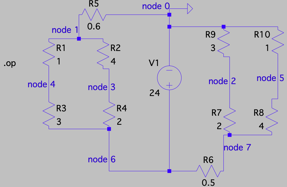
R1 N001 N004 1
R2 N001 N003 4 R3 N004 N006 3 R4 N003 N006 2 R5 0 N001 0.6 R6 N007 N006 0.5 R7 N007 N002 2 R8 N007 N005 4 R9 N002 0 3 R10 N005 0 1 V1 N006 0 24 .op .backanno .end |
Equivalent Resistance
|
V(n001) 4.8
V(n004) 9.6 V(n003) 17.6 V(n006) 24 V(n007) 20 V(n002) 12 V(n005) 4 I(R10) 4 I(R9) 4 I(R8) 4 I(R7) 4 I(R6) -8 I(R5) -8 I(R4) -3.2 I(R3) -4.8 I(R2) -3.2 I(R1) -4.8 I(V1) -16 |
One of the first test circuits that worked – a single voltage source, grounded at the negative end, and a net of resistors. Essentially measuring the equivalent resistance across a finite set of resistors. |
|
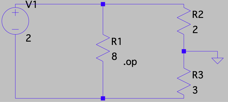
R1 N001 N002 8
R2 N001 0 2 R3 0 N002 3 V1 N001 N002 2 .op .backanno .end |
Parallel Voltage
|
V(n001) 0.8
V(n002) -1.2 I(R3) -0.4 I(R2) -0.4 I(R1) -0.25 I(V1) -0.65 |
One of the earliest tests - the first version of the code could only handle one voltage source, with the ground at the negative end. This circuit tested the ability to place the ground anywhere. |
|
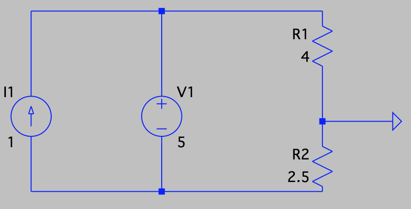
R1 N002 0 4
R2 N001 0 2.5 V1 N002 N001 5 I1 N001 N002 1 .op .backanno .end |
Parallel Sources
|
V(n002) 3.077
V(n001) -1.923 I(I1) 1 I(R2) -0.769 I(R1) 0.769 I(V1) 0.231 |
A lot of work had to happen to allow multiple sources to be added, especially current sources, and especially sources linked together. This simple circuit tests a lot of essential implementation details. |
|
V3 N001 P001 1
I1 0 P001 2 V4 N001 P002 4 R1 P002 0 1 I2 N001 0 1 V2 P003 0 1 R2 N001 P003 4.7 R3 N001 P004 1.5 R4 P004 0 2 .op .backanno .end |
Many Sources
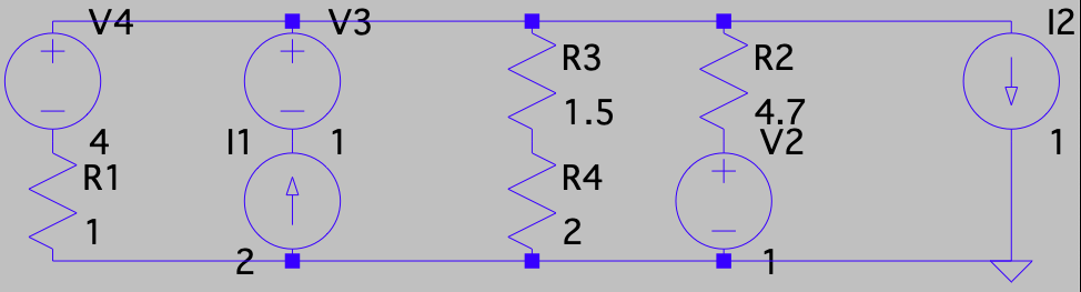
|
V(p003) 1
V(n001) 3.479 V(p001) 2.479 V(p002) -0.521 V(p004) 1.988 I(I2) 1 I(I1) 2 I(R4) 0.994 I(R3) 0.994 I(R2) 0.527 I(R1) -0.521 I(V4) -0.521 I(V3) -2 I(V2) 0.527 |
A stress test of the implementation of the sources. |
|
R2 N003 N004 2
R3 0 N001 2 R4 N003 0 1 C1 N003 N003 0.0001 V2 N001 N002 0.5 V1 N002 N004 1.5 .op .backanno .end |
Shorted Capacitor
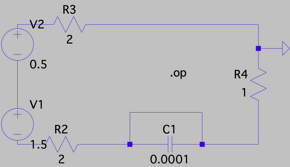
|
V(n002) 0.3
V(n004) -1.2 V(n001) 0.8 V(n003) -0.4 I(R4) 0.4 I(R3) 0.4 I(R2) -0.4 I(V2) -0.4 I(V1) -0.4 |
This tests an edge case - what happens when a component is shorted. |
|
R1 N011 N015 0.007
R2 0 N015 10 R3 N002 0 1 R4 N001 N004 2 R5 N010 N015 0.5 R6 N015 N014 5.1 R7 N014 N008 1.7 R8 N006 N001 1.5 R9 P001 N001 4 R10 N007 N012 4 R11 N013 N014 4 R12 N016 N014 5 R13 N002 N001 4 R14 N003 N005 1 I1 P001 N003 2 I2 N002 N011 1 R15 N003 N005 2 C1 N001 N009 0.001 C2 N004 N010 0.001 C3 N006 N008 50 L1 N012 N016 0.5 L2 N007 N013 1 L3 N009 N015 4 V1 N001 N014 5 V2 N005 N007 5 .op .backanno .end |
Multi-Source RLC
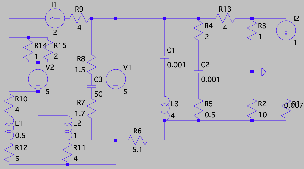
|
V(n011) 2.0468
V(n015) 2.0398 V(n002) -0.204 V(n001) 2.980 V(n004) 2.980 V(n010) 2.0398 V(n014) -2.0199 V(n008) -2.0199 V(n006) 2.9801 V(p001) -5.0199 V(n007) 3.520 V(n012) 1.0579 V(n013) 3.518 V(n016) 1.0573 V(n003) 9.853 V(n005) 8.520 V(n009) 2.0398 I(C3) 2.5e-10 I(C2) 9.403e-16 I(C1) 9.403e-16 I(L3) 0 I(L2) 1.385 I(L1) 0.615 I(I2) 1 I(I1) 2 I(R15) 0.667 I(R14) 1.333 I(R13) -0.796 I(R12) 0.615 I(R11) 1.385 I(R10) 0.615 I(R9) -2 I(R8) -2.5e-10 I(R7) -2.5e-10 I(R6) 0.796 I(R5) 8.882e-16 I(R4) 6.661e-16 I(R3) -0.204 I(R2) -0.204 I(R1) 1 I(V2) 2 I(V1) -2.796 |
A full test of an RLC circuit, with multiples of everything including the sources, and multiple supernodes of different types. |
|
R2 N003 0 3
D1 N002 N003 D V1 N001 N004 7 R1 N002 N001 2 R3 0 N004 1 .lib ~/Library/Application Support/LTspice/lib/cmp/standard.dio .op .backanno .end |
Diode
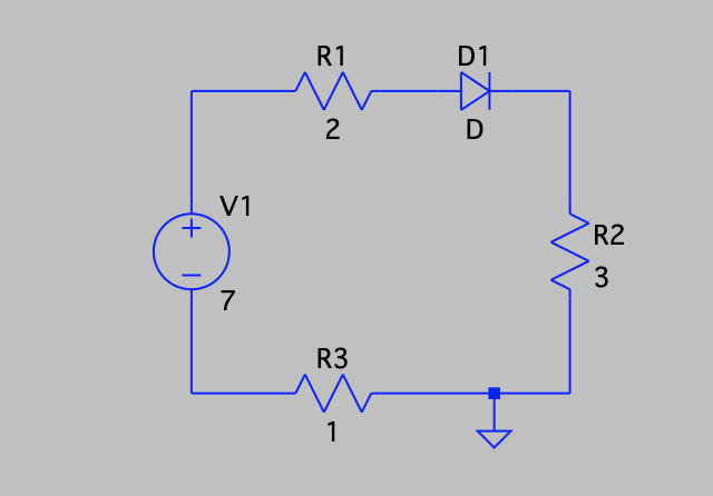
|
V(n003) 3.08275
V(n002) 3.91725 V(n001) 5.97242 V(n004) -1.02758 I(D1) 1.02759 I(R3) 1.02758 I(R1) -1.02758 I(R2) 1.02758 I(V1) -1.02758 |
As a final step, a nonlinear component was implemented to verify the solver. A very simple circuit with a diode included, as a verification of the diode implementation. The voltage across the diode differs from LTspice by ~1%, no doubt because LTspice uses a 17- parameter Berkeley diode model and I am just using the 3-parameter Shockley equation. |
|
V1 N002 N012 5
V2 N005 N007 5 I1 P001 N001 2 I2 N003 N010 1 L1 P002 P003 0.5 L2 N007 P004 1 L3 N008 N011 4 C1 N002 N008 0.001 C3 P005 P006 50 R1 N010 N011 0.007 R2 0 N011 10 R3 N003 0 1 R4 N002 N006 2 R5 N009 N011 0.5 R6 N011 N012 5.1 R7 N012 P006 1.7 R8 P005 N002 1.5 R9 P001 N002 4 R10 N007 P002 4 R11 P004 N012 4 R12 P003 N012 5 R13 N003 N002 4 R15 N001 N005 2 D1 N006 N009 D D2 N001 N004 D R14 N005 N004 1 L4 N015 N012 0.5 D3 N011 N015 D V3 N014 N013 4 D4 N014 N011 D R16 N011 N013 4 .model D D .lib ~/Library/Application Support/LTspice/lib/cmp/standard.dio .op .backanno .end |
RLC with Diodes
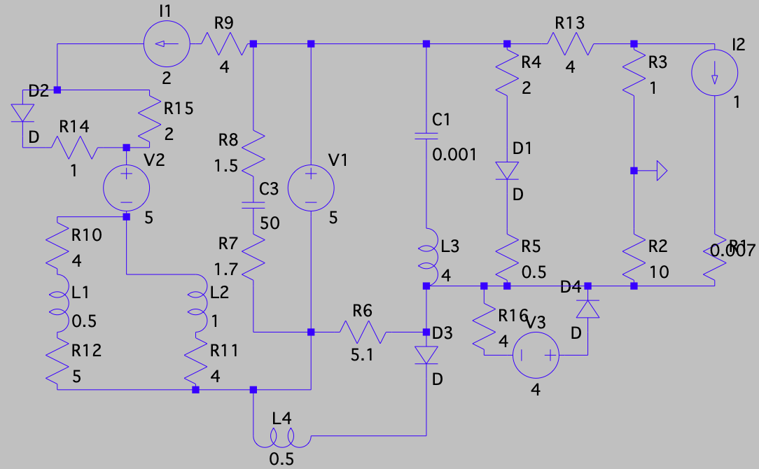
|
V(n002) 4.048
V(n012) -0.9520 V(n005) 9.588 V(n007) 4.588 V(p001) -3.952 V(n001) 11.478 V(n003) 0.00961 V(n010) -0.0891 V(p002) 2.126 V(p003) 2.125 V(p004) 4.586 V(n008) -0.0961 V(n011) -0.0961 V(p005) 4.0480 V(p006) -0.952 V(n006) 1.406 V(n009) 0.565 V(n004) 10.643 V(n015) -0.950 V(n014) 0.732 V(n013) -3.268 I(C3) 2.5e-10 I(C1) 4.144e-15 I(D4) 0.793 I(D3) 2.163 I(D2) 1.0549 I(D1) 1.321 I(L4) 2.163 I(L3) 0 I(L2) 1.385 I(L1) 0.615 I(I2) 1 I(I1) 2 I(R16) 0.793 I(R14) -1.0549 I(R15) 0.945 I(R13) -1.00961 I(R12) 0.615 I(R11) 1.385 I(R10) 0.615 I(R9) -2 I(R8) -2.5e-10 I(R7) -2.5e-10 I(R6) 0.168 I(R5) 1.321 I(R4) 1.321 I(R3) 0.00961 I(R2) 0.00961 I(R1) 1 I(V3) -0.793 I(V2) 2 I(V1) -4.331 |
Final test - a messy circuit with multiples of all implemented components. Some of the values differ from LTspice by a few %, because the diode models are different. |